文章目录 [隐藏]
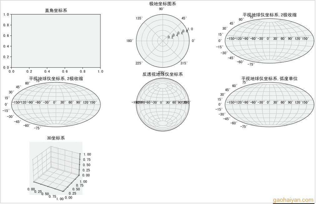
1.matplot的坐标系
|
1 2 3 4 5 6 7 8 9 10 11 12 13 14 15 16 17 18 19 20 21 22 23 24 25 26 27 28 29 30 31 32 33 34 35 36 37 38 39 40 41 42 43 |
import matplotlib.pyplot as plt # matplot的坐标系projection有这些: # from matplotlib.projections import axes # from matplotlib.projections.geo import AitoffAxes, HammerAxes, LambertAxes, MollweideAxes # from matplotlib.projections.polar import PolarAxes # from mpl_toolkits.mplot3d import Axes3D # # print(axes.Axes.name) # rectilinear 直角坐标 # print(PolarAxes.name) # polar 极地坐标图 # print(AitoffAxes.name) # aitoff 平视地球仪坐标:上下2极收缩 # print(HammerAxes.name) # hammer 平视地球仪坐标:上下2极收缩 # print(LambertAxes.name) # lambert 反透视地球仪坐标:上下2极收缩到圆内 # print(MollweideAxes.name) # mollweide 平视地球仪坐标:数据单位必须是弧度 # print(Axes3D.name) # 3d 3D坐标图 ax1 = plt.subplot(3, 3, 1, facecolor="#eeefef", projection='rectilinear') ax1.set_title("直角坐标系") ax2 = plt.subplot(3, 3, 2, facecolor="#eeefef", projection='polar') ax2.set_title("极地坐标图系") ax3 = plt.subplot(3, 3, 3, facecolor="#eeefef", projection='aitoff') ax3.set_title("平视地球仪坐标系,2极收缩") ax3.grid() ax4 = plt.subplot(3, 3, 4, facecolor="#eeefef", projection='hammer') ax4.set_title("平视地球仪坐标系,2极收缩") ax4.grid() ax5 = plt.subplot(3, 3, 5, facecolor="#eeefef", projection='lambert') ax5.set_title("反透视地球仪坐标系") ax5.grid() ax6 = plt.subplot(3, 3, 6, facecolor="#eeefef", projection='mollweide') ax6.set_title("平视地球仪坐标系,弧度单位") ax6.grid() ax7 = plt.subplot(3, 3, 7, facecolor="#eeefef", projection='3d') ax7.set_title("3D坐标系") plt.show() |
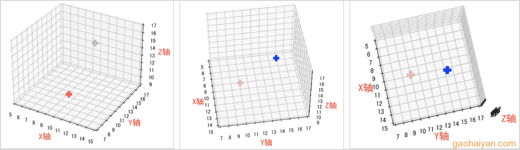
2.三维空间图形-点
|
1 2 3 4 5 6 7 8 9 10 11 12 13 14 15 16 17 18 19 20 21 22 23 24 25 26 27 28 29 30 31 32 33 34 35 |
import matplotlib.pyplot as plt from matplotlib.pyplot import MultipleLocator from mpl_toolkits.mplot3d import Axes3D # 空间三维画图 # pycharm中的matplotliib 3D图旋转设置 # Settings,找到“Python Scientific”,去除勾选“Show plots in toolwindow” fig = plt.figure(5) ax = fig.add_subplot(1, 1, 1, projection='3d') # 绘制三维图 ax.set_xlim(5, 15) ax.set_ylim(7, 17) ax.set_zlim(9, 17) ax.xaxis.set_major_locator(MultipleLocator(1)) ax.yaxis.set_major_locator(MultipleLocator(1)) ax.zaxis.set_major_locator(MultipleLocator(1)) ax.set_zlabel('Z轴', fontdict={'size': 15, 'color': 'red'}) ax.set_ylabel('Y轴', fontdict={'size': 15, 'color': 'red'}) ax.set_xlabel('X轴', fontdict={'size': 15, 'color': 'red'}) # 3D空间的点 # x1 = [6] # y1 = [9] # z1 = [10] # ax = Axes3D(fig) # ax.scatter(x1, y1, z1, marker="D", c='b', label='A3D点') # ax.legend(loc='best')# 绘制图例 # 3D空间的点 # 2个点数据。(10,10,10) (11,14,15)。默认离得远的会透明化 x = [10, 11] y = [10, 14] z = [10, 15] ax.scatter(x, y, z, marker='P', s=120, c=['#ff3333', '#0000ff']) plt.show() |
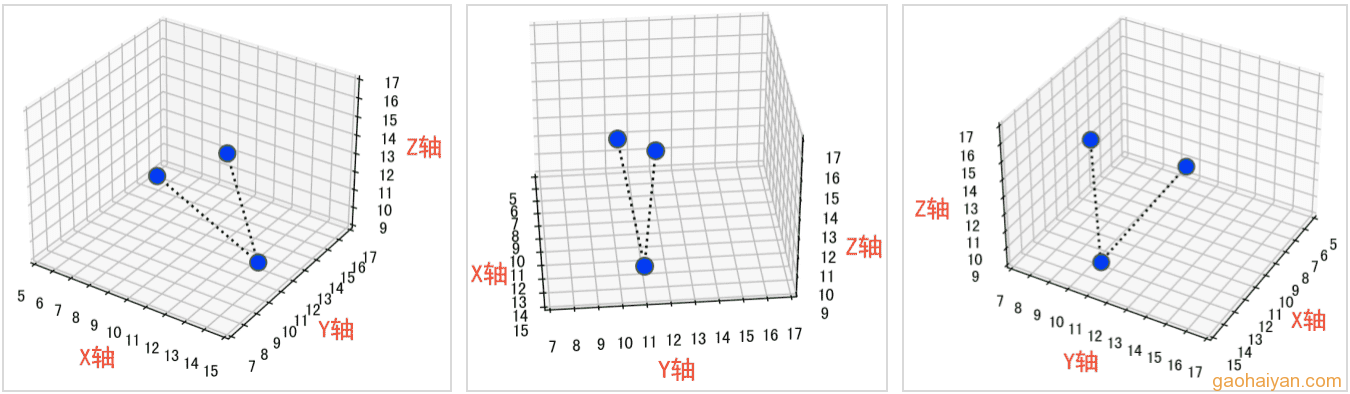
3.三维空间图形-线
|
1 2 3 4 5 6 7 8 9 10 11 12 13 14 15 16 17 18 |
import matplotlib.pyplot as plt fig = plt.figure() ax = fig.add_subplot(1, 1, 1, projection='3d') # 绘制三维图 ax.plot3D( xs=[8, 14, 13], # x 轴坐标 ys=[12, 11, 10], # y 轴坐标 zs=[12, 10, 16], # z 轴坐标 ls=':', # 线条样式 color='k', # 线条颜色 marker='o', # 标记样式 mfc='b', # 标记颜色 mec='g', # 标记描边颜色 ms=10, # 标记大小 ) plt.show() |
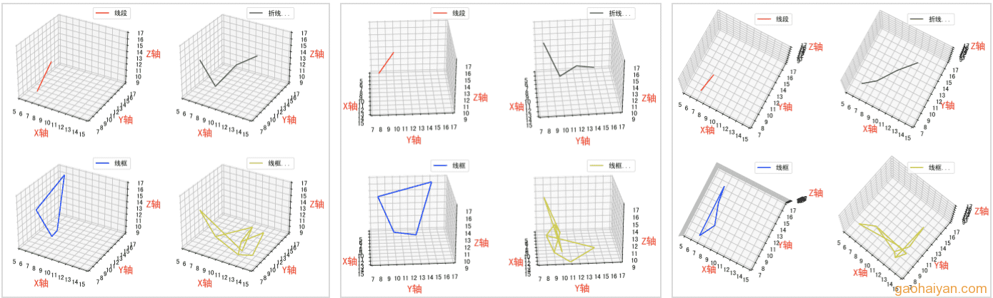
4.三维空间图形-线框
|
1 2 3 4 5 6 7 8 9 10 11 12 13 14 15 16 17 18 19 20 21 22 23 24 25 26 27 28 29 30 31 32 33 34 35 36 37 38 39 40 41 42 43 44 45 46 47 48 |
import matplotlib.pyplot as plt import numpy as np from matplotlib.pyplot import MultipleLocator # 线段 x1 = [[7, 8]] y1 = [[8, 10]] z1 = np.array([[10, 14]]) # 须要转为numpy的列表,否则:axes3d.py", line 1555, in plot_surface if Z.ndim != 2: AttributeError: 'list' object has no attribute 'ndim' # 折线 x2 = [[7, 8, 10]] y2 = [[8, 10, 12]] z2 = np.array([[15, 10, 13]]) # 折线... x2 = [[7, 8, 10, 12]] y2 = [[8, 10, 12, 14]] z2 = np.array([[15, 10, 13, 14]]) # 封闭的线框 x3 = [[7, 8], # [7, 7]] y3 = [[8, 10], # [15, 13]] z3 = np.array([[15, 10], [17, 9]]) # 封闭的线框... x4 = [[7, 8, 12, 13], # [12, 14, 13, 13]] y4 = [[8, 10, 9, 11], # [10, 9, 8, 14]] z4 = np.array([[15, 10, 9, 8], # [9, 14, 12, 10]]) ax1 = fig.add_subplot(2, 2, 1, projection='3d') ax2 = fig.add_subplot(2, 2, 2, projection='3d') ax3 = fig.add_subplot(2, 2, 3, projection='3d') ax4 = fig.add_subplot(2, 2, 4, projection='3d') ax1.plot_wireframe(X=x1, Y=y1, Z=z1, color='r', label='线段') ax2.plot_wireframe(X=x2, Y=y2, Z=z2, color='g', label='折线...') ax3.plot_wireframe(X=x3, Y=y3, Z=z3, color='b', label='线框') ax4.plot_wireframe(X=x4, Y=y4, Z=z4, color='y', label='线框...') ax1.legend() ax2.legend() ax3.legend() ax4.legend() plt.show() |
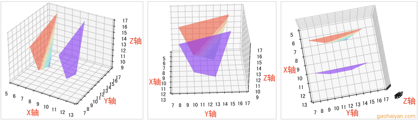
5.三维空间图形-面和投影
|
1 2 3 4 5 6 7 8 9 10 11 12 13 14 15 16 17 18 19 20 21 22 23 24 25 26 27 28 29 30 31 32 33 34 35 36 37 38 39 40 41 42 |
import numpy as np import matplotlib.pyplot as plt from matplotlib import cm # 面的着色支持的颜色有: cmaps = cm.cmap_d.keys() for color in cmaps: print(color) # 3D空间的面。至少4个顶点。要求顶点个数为 2n 或 n^2 # 四边形的4个顶点(a, h, m]) (b, i, n) (c, j, o) (d, k, p) x = [ # x轴的4个点,数值大体上相同,即3d面是(大体上)垂直于x轴的yz面 # 如果要用contourf方法对面进行投影,数值完全相同时,作为zdird的轴,会导致:art3d.py, line 769, in do_3d_projection zip(*z_segments_2d) ValueError: not enough values to unpack (expected 5, got 0) [10.5, 10.5], # a, b [10.5, 10.4]] # c, d y = [ # y轴4个点 [8, 10], # h, i [15, 13]] # j, k z = np.array( # 须要转为numpy的列表,否则:axes3d.py", line 1555, in plot_surface if Z.ndim != 2: AttributeError: 'list' object has no attribute 'ndim' [ # z轴4个点。 [15, 10], # m, n [17, 9]]) # o, p ax.plot_surface( # X=x, Y=y, Z=z, color='g', alpha=0.6, # rstride=1, # 对应x轴,行之间的跨度。大于0整数,默认1。影响面的平滑度,值越大越粗糙。 # cstride=1, # 对应y轴,列之间的跨度。简单理解:某个轴有n个点,n/r(c)stride即为显示的个数 cmap='rainbow' # 面的着色。彩虹 rainbow、热度 coolwarm ) # 对surface面进行投影 ax.contourf(# x, y, z,# alpha=0.6, # zdir='x', # zdir指以哪个轴投影。如z,即将影子投在xy平面上 offset=7, # 将影子投射到 zdir 轴的某个刻度。影子是个平面,垂直于zdir轴 cmap='rainbow') plt.show() |
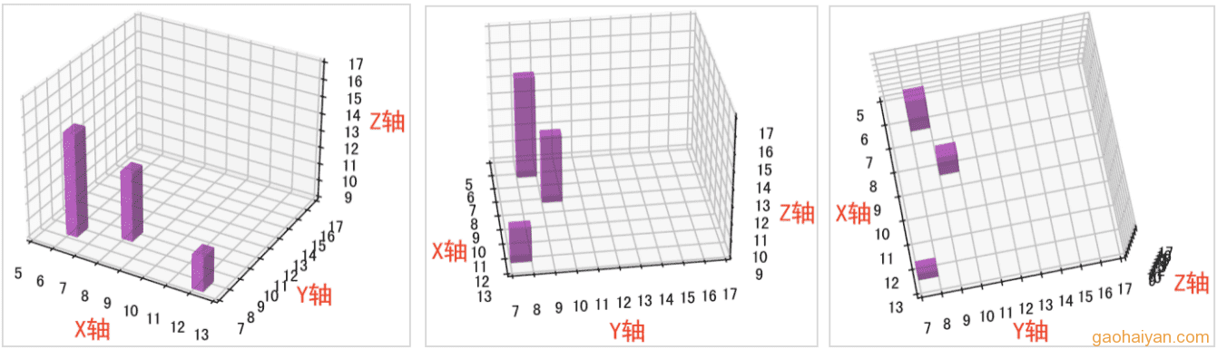
6.三维空间图形-立体柱子
|
1 2 3 4 5 6 7 8 9 10 11 12 13 14 15 16 17 18 19 |
import matplotlib.pyplot as plt x_pos = [8, 12, 6] y_pos = [9, 7, 8] z_pos = [9, 9, 9] # 都在xy轴的平面上 x_width = 0.5 # x轴上的长度 y_width = 1 # y轴上的宽度 z_height = [4, 2, 6] # z轴上的高度。顶部位置 = z_pos + z_height ax.bar3d( # x=x_pos, # y=y_pos, # z=z_pos, # dx=x_width, # dy=y_width, # dz=z_height, # color='m', # alpha=0.5) plt.show() |
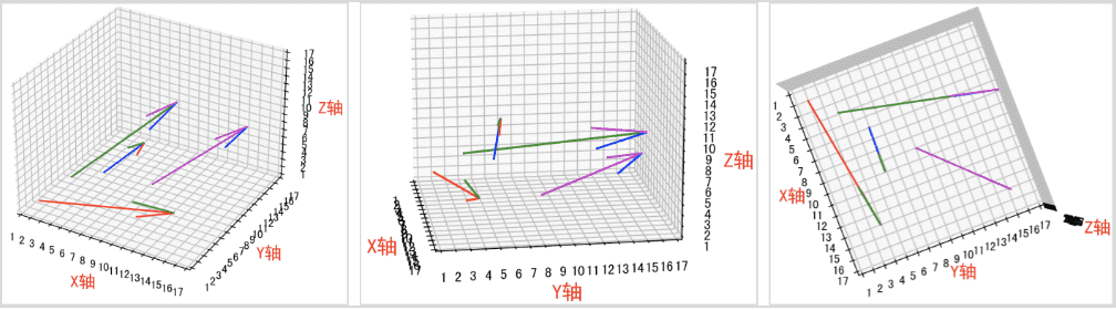
7.三维空间图形-矢量场-风向标
|
1 2 3 4 5 6 7 8 9 10 11 12 13 14 15 16 17 18 19 20 |
import matplotlib.pyplot as plt fig = plt.figure() ax = fig.add_subplot(1, 1, 1, projection='3d') # 绘制三维图 x = [[[2, 4], [6, 9]]] y = [[[2, 4], [6, 9]]] z = [[[2, 4.5], [4.5, 2]]] u = [[[14-2, 7-4], [10-6, 15-9]]] v = [[[4-2, 17-4], [6-6, 15-9]]] w = [[[4-2, 7-4.5], [10-4.5, 8-2]]] ax.quiver(x, y, z, # 箭头的位置-尾巴的 u, v, w, # 箭头的指向-尖头的 x y z color=['r', 'g', 'b', 'm'], # 颜色 length=1, # 箭头长度百分比。(uvw + xyz) * length normalize=False)# 是否将所有箭头规格化为具有相同的长度。默认True,一个刻度长度。 plt.show() |
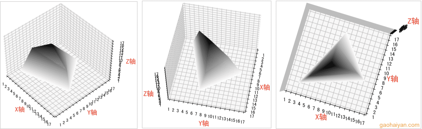
8.三维空间图形-等高线
|
1 2 3 4 5 6 7 8 9 10 11 12 13 14 15 16 17 18 19 20 21 22 23 24 |
import matplotlib.pyplot as plt from matplotlib.pyplot import MultipleLocator # 第1维元素:山脊或山坳数量。手动设置的线越多,山势细节越多 # 第2维元素:从山脚到山顶,设置2道等高线。中间的根据contour第4个参数细密度补齐 x = [[3, 5], [15, 13], [9, 8], [3, 5]] y = [[3, 5], [7, 8], [15, 12], [3, 5]] z = [[3, 15], [3, 16], [3, 16], [3, 15]] # 第2维:设置3道等高线。手动设置的线越多,山势细节越多 x = [[3, 5, 8], [15, 13, 8], [9, 8, 8], [3, 5, 8]] y = [[3, 5, 8], [7, 8, 8], [15, 12, 8], [3, 5, 8]] z = [[3, 13, 15], [3, 9, 15], [3, 8, 15], [3, 13, 15]] fig = plt.figure() ax = fig.add_subplot(1, 1, 1, projection='3d') ax.contour( x, # y, # z, # 顶点位置 60, # 细密度。默认5 cmap='binary') # 着色 plt.show() |
- end
声明
本文由崔维友 威格灵 cuiweiyou vigiles cuiweiyou 原创,转载请注明出处:http://www.gaohaiyan.com/2990.html
承接App定制、企业web站点、办公系统软件 设计开发,外包项目,毕设


